
1. Calculated Fields
Creating a Calculated Field
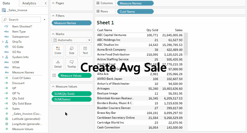
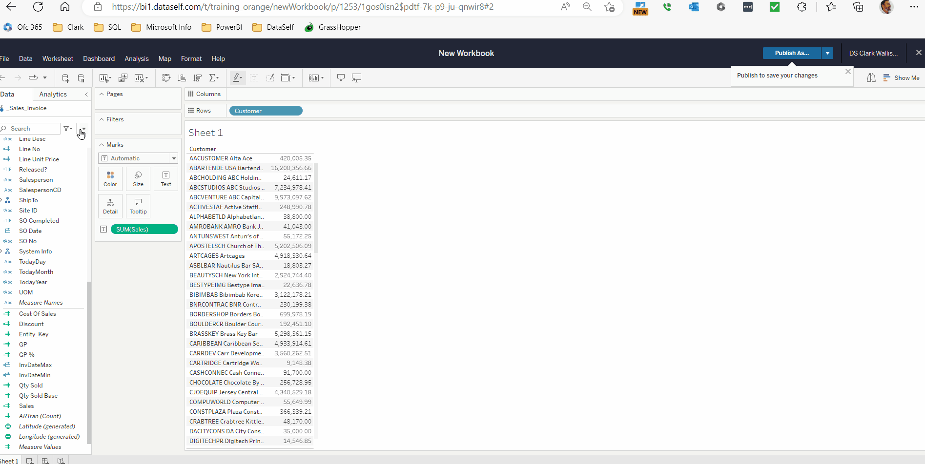
Activity 1: Create a new worksheet with Item , Sales, and Qty Sold.
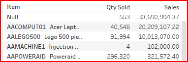
Then create a calculated field, Avg Unit Sales = Sales divided by Qty Sold:
-
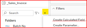
On the left pane, click the down arrow by the Search box and select Create Calculated Field.
-
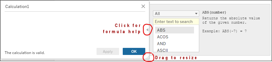
Type in the field name: Avg Unit Sales.
-
Enter in the expression area: [Sales]/[Qty Sold]
-
Check the output of the calculation. It is not what you expect when you manually calculate the value of Sales / Qty Sold on the screen.
-
-
Change the calculation to: SUM([Sales])/SUM([Qty Sold]).
-
Check the output of the calculation. This should match your manual calculation of Sales / Qty Sold.
-
To see information about function, SUM(), Click the > right arrow icon on the right of the calculation window, find the function SUM() and click the function name to learn details.
To resize the expression area: drag the bottom-right corner of the pop up.
Click Ok.
What’s the difference between [Sales] / [Qty Sold] and Sum([Sales]) / Sum ([Qty Sold])?
Without the Sum aggregation function, Tableau will do the division for each transaction line then display the sum of the transaction level results. The measure value will show SUM then the calculation by default.
With the SUM aggregation functions for each field in the calculation, Tableau will do the division with the summary amounts, not individual transaction records. The measure function will show AGG then the calculation, indicating the aggregation is built into the calculation. To format the number, click the down arrow on the green field in the Measures Value section→ Format Number. Select the format as desired.
-

Note the difference between the SUM and AGG on the Measure Values
Examples of Measure Calculations
The following are insightful examples of measure expressions:
-
Sales before Discount = Sales plus Discount.
-
SUM([Sales]) + SUM ([Discount])
-
-
Avg Price = Sales divided by Qty Sold.
-
SUM([Sales]) / SUM ([Qty Sold])
-
-
Avg Sale per Invoice = Sales divided by the number of invoices.
-
SUM([Sales]) / COUNTD ([Inv No])
-
-
Avg Sale per Transaction = Sales divided by number or transaction lines:
-
SUM([Sales]) / COUNT ([_Sales_Invoice])
-
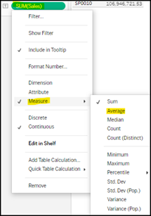
Alternatively, drag Sales to a report, right-click the Sales green pill on the center panel → Measure → Average.
-
-
Max Individual Sale Price.
-
MAX([Sales])
-
Alternatively, drag Sales to a report, right-click the Sales green pill on the center panel → Measure → Maximum.
-
Tableau’s version of Averages
-
One way to do averages is to change the measure's aggregation type by right clicking on the measure in the Measure Values section then selecting Measures and Average. This built in Average calculates the Sum divided by number of transaction records. That’s not always what you want, which is why we show how to do your own average calculations.
Conditional Measure Calculations (for reference)
Tableau help on logical functions:
The following are examples of common conditional expressions:
-
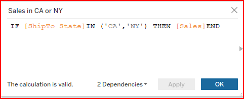
Sales in ShipTo State = CA or NY.
-
Tableau builds in the ELSE = NULL logic for you, so you don’t have to write it.
-
IF [ShipTo State] = 'CA' OR [ShipTo State] = 'NY' THEN [Sales] END
-
-
Expression 2 with zero for other states:
-
IF [ShipTo State] = 'CA' OR [ShipTo State] = 'NY' THEN [Sales] ELSE 0 END
-
-
Doing if / then with multiple conditions using the
INoperator offers more flexibility.-
IF [ShipTo State] IN ('CA', ‘NY’) THEN [Sales] END
-
-
Using the
NOToperator selects when the multiple conditions are NOT met.-
IF NOT ([ShipTo State]) IN ('CA', ‘NY’) THEN [Sales] END
-
-
-
Division by Zero
-
If the denominator is zero, then return a given value (99.9 in the example below).
(Tableau default division by zero result is NULL)-
IF SUM([Cost Of Sales])=0 then 99.9 else SUM([Sales])/SUM([Cost Of Sales]) END
-
-
-
Handling NULLs
-
Formula ZN returns expression if not NULL, otherwise returns zero:
Important because you can’t do math with NULL values-
ZN([Cost Of Sales])
-
-
Formula IFNULL returns expression if not NULL, otherwise returns the 2nd parameter:
-
IFNULL([Cost Of Sales],1)
-
-
Activity 2: Conditional Sales Measure Ship-To States of CA or NY
-
Create a worksheet showing the Customer Dimension and the Sales Measure
-
Create a Calculated Measure showing Sales when the Ship To State is equal to ‘CA’ or ‘NY’.
The screenshots below show two different ways of creating the calculation.
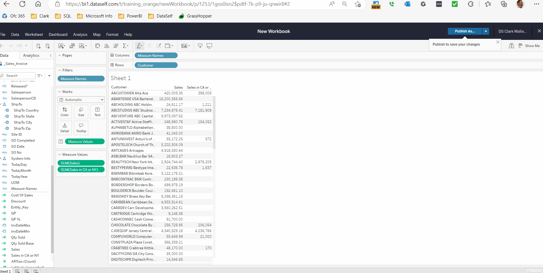
Create a calculated field showing sales not in CA or NY. Sum([Sales]) - Sum([Sales in CA or NY])
Notice that on rows where there is no CA/NY sales, there is nothing in the calculated field Sales not in CA or NY. This because Tableau cannot calculate a NULL value. You can use the ZN function to convert the NULL value to a ZERO value. Then Tableau can calculate it.
Change the calculation to show Sum([Sales]) - ZN(Sum(Sales in CA or NY])).
The calculated measure for Sales not in CA or NY should now show values for all rows.
Other Conditional Measure Calculations (for reference)
-
Sales in a Given Period
-
Fixed year = 2021:
-
IF YEAR([Inv Date])=2021 THEN [Sales] END
-
-
Fixed fiscal year FY 2021:
-
IF [FYear No]=2021 THEN [Sales] END
-
IF [FYear]='FY 2021' THEN [Sales] END
-
-
Relative year = This Year:
-
IF YEAR([Inv Date])=YEAR(TODAY()) THEN [Sales] END
-
-
Relative fiscal year = This FYear:
-
IF [Relative FYr]=0 THEN [Sales] END
-
-
Relative year = Last Year:
-
IF YEAR([Inv Date])=YEAR(TODAY())-1 THEN [Sales] END
-
-
Relative fiscal year = Last FYear:
-
IF [Relative FYr]=-1 THEN [Sales] END
-
-
Relative fiscal YTD = Last Fiscal YTD
-
IF [Relative FYr]=-1 AND [YTD Fiscal]='YTD' THEN [Sales] END
-
-
Relative month = Same Month Last Year
-
IF YEAR([Inv Date])=YEAR(TODAY())-1 AND MONTH([Inv Date])=MONTH(TODAY()) THEN [Sales] END
-
IF [Relative FMo]=-12 THEN [Sales] END
-
-
-
Growth (using ZN())
-
Sales in FY 2021 minus FY 2020
-
ZN(IF [FYear No]=2021 THEN [Sales] END) - ZN(IF [FYear No]=2020 THEN [Sales] END)
-
Important: Tableau returns NULL if a value in an expression is NULL. For instance, if a customer had no transactions last year (NULL value) and $100 sales this year, Tableau returns sales growth of $100 - NULL = NULL. Use formula ZN to process ZN($100)-ZN(NULL)=$100.
-
-
-
Growth %
-
(Sales in FY 2021 minus FY 2020) / (Sales in FY 2020), returning NULL if FY 2020 Sales is NULL or zero.
-
if ZN(IF [FYear No]=2020 THEN [Sales] END) = 0 then NULL else (ZN(IF [FYear No]=2021 THEN [Sales] END) - ZN(IF [FYear No]=2020 THEN [Sales] END)) / ZN(IF [FYear No]=2020 THEN [Sales] END).
-
-
Help topics for aggregated vs non-aggregated measure errors:
-
Cannot mix aggregate and non-aggregate arguments with this function.
-
Using aggregated measures in if / then statements. Basic rule - write the conditional statement first, then add the aggregation to the beginning with () around the conditional statement
Dimension Calculated Expressions (for reference)
The following are insightful examples of dimension expressions:
-
Combining character fields: Inv Type ID + Inv No.
-
[Inv Type ID]+' - '+[Inv No]
-
-
The left part of a string:
-
LEFT([Inv No],2)
-
Examples:
-
The main section of Item IDs comprised of the first 4 digits: LEFT([Item ID],4)
-
The 1st segment of a GL account comprised of the first 5 digits: LEFT([GL Account],5)
-
-
-
A subset of a string:
-
MID([Inv No],3,2)
-
Examples:
-
The 2nd segment of Item IDs, starting at digit 5, 3 digits long: MID([Item ID],5,3)
-
The 2nd segment of a GL account, starting at digit 6, 2 digits long: MID([GL Account],6,2)
-
-
-
The right part of a string:
-
RIGHT([Inv No],2)
-
-
Converting an expression to a string:
-
‘FY ’+STR([FYear No])
-
Calculated Fields for Filters (True|False)
You can create calculated fields to filter data. The following are some popular concepts. Drag and drop the calculated field in the Filters section and set it for TRUE (or FALSE).
-
Filtering for some members of a dimension:
-
[ShipTo State]='NY'
-
-
Filtering for members that contain a certain string:
-
CONTAINS([Customer],'Starbuckets')
-
-
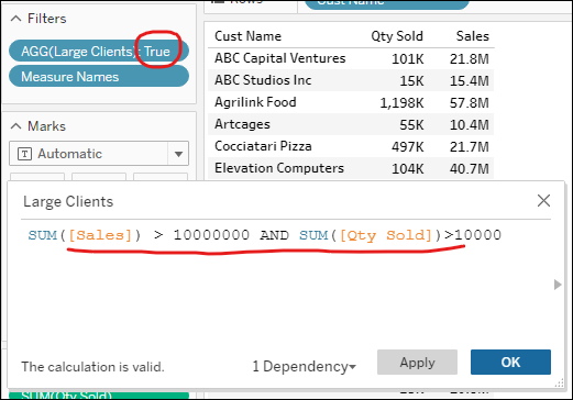
Filtering for members that meet a certain measure criteria:
-
SUM([Sales]) > 1000 AND SUM([Qty Sold])>100
-
2. Quick Table Calculations
Quick table calculations allow to quickly apply a common table calculation to your visualization using the most typical settings for that calculation type.
Creating Quick Table Calculations
-
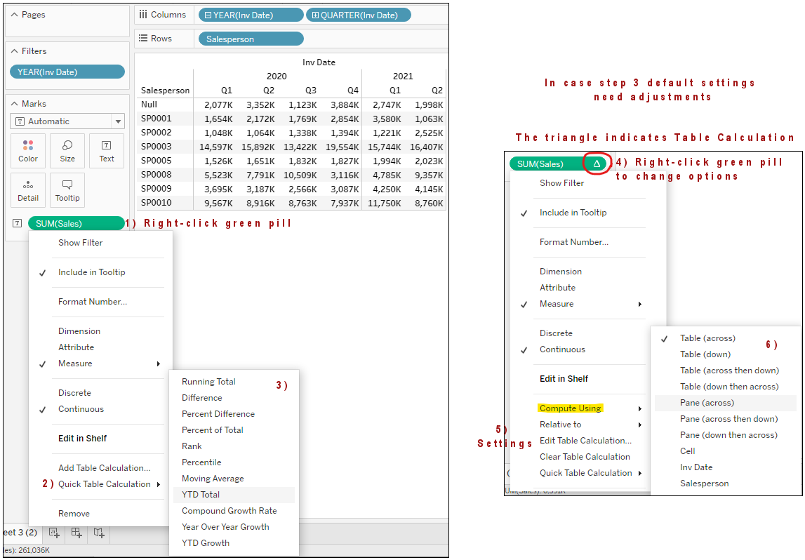
Right-click the green field of a report measure → Quick Table Calculation → select an option.
-
Some options might be disabled depending on the report (ex.: some of them require a date field).
-
Build the report below to explore the options.
-
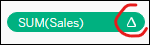
Report measures using Table Calculations show a triangle on their green fields. See below.
-
In many cases, step 3 works right off the bat. When it doesn’t, explore steps 4, 5 and 6.
-
For instance, you might want to use a Quick Table Calculation working Table (across) but step 3 created one working Tableau (down). In this case, go to step 4 → Compute Using → Table (down).
-
Quick Table Calculations: Generic Types
-
Running Total: The accumulated total by rows or columns. Ex.: cell 1 = 100, cell 2 = 50 value, cell 3 = 150, the Running Total: cell 1 = 100, cell 2 = 150, cell 3 = 300.
-
Difference: The difference between two cells by rows or columns. Ex.: same example as above, the Difference will have cell 1 = NULL, cell 2 = 50, cell 3 = 100.
-
Percent Difference: The % difference between two cells by rows or columns. Ex.: same example as above, the % Difference will have cell 1 = NULL, cell 2 = 50%, cell 3 = 200%.
-
Percent of Total: The % total of all cells by rows or columns. Ex.: same example as above, the % of Total will have cell 1 = 33.3%, cell 2 = 16.6%, cell 3 = 50%.
-
Rank: The rank of a cell based on rows or columns. Ex.: same example as above, the Rank will have cell 1 = 2, cell 2 = 3, cell 3 = 1.
-
Percentile: For each mark in the view, a Percentile table calculation computes a percentile rank for each value in a partition. Ex.: same example as above, the Percentile will have cell 1 = 50%, cell 2 = 0, cell 3 = 100%.
-
Moving Average: For each mark in the view, it calculates the value by performing the average across a specified number of values before and/or after the current value. Ex.: same example as above, the 2 cell Moving Avg will have cell 1 = 100, cell 2 = 75, cell 3 = 100.
Quick Table Calculations: Date Dependent (for reference)
-
YTD Total: The same as Running Total, requires a date field and resets the running total every year.
-
Compound Growth Rate: Accumulates the growth rate by period divided by (number of cells minus 1).
-
Year Over Year Growth: Calculates the growth from the same period in prior year.
-
YTD Growth: Calculates the YTD growth from the prior year.
Tableau Help:
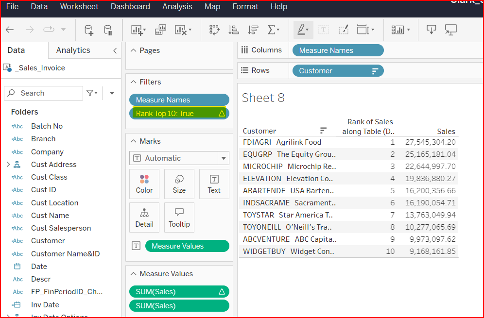
Activity 3: Create worksheet with Top 10 Customers Ranked by Sales
Create a new worksheet with the Customer dimension and Sales measure.
Change the Sum([Sales]) measure to a Rank Table Calculation, then add the Sum([Sales]) measure back to the measure values section. Make sure the Rank Table Calculation scans down the table, not across.
Sort the Sales Measure in Descending order. The Sales should show from highest to lowest, and the rank from lowest to highest. You should now see the customers sorted in Rank order.
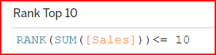
Drag the Rank Table Calculation measure to the data pane. The cursor should show a + sign indicating it will add it as a new calculated field. It will automatically name it something like Calculation 1.
Edit the calculation, renaming it to Rank Top 10 and adding <= 10 to the end of the calculation.
The calculated field should now look like this:
This is now a True|False field that can be used as a Filter. Drag the calculated field to the filters section and select only True. Now you see only the Top 10 sales customers.
3. Parameters
User-defined parameters can be used in calculated fields, filters and other report structures. They provide users with the ability to change values in an user-friendly way.
Here’s how to create and show parameters in reports:
-
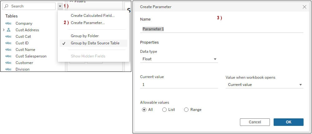
Click the arrow down by the Search box on the data panel → Create Parameter → select the parameter options → Ok.
-
Parameters are listed at the bottom of the Data panel.
-
To show Parameters on reports, right-click on a parameter name → Show Parameter. The parameter will be posted on the right panel of a report.
Optional Hands-on Exercises
The following are insightful hands-on exercises using parameters and calculated fields:
-
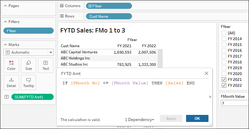
FYTD Calculation Using Parameter for the Month Number:
-
Create a parameter named FMonth Value, with Type = Integer.
-
Create a calculated field: IF [FMonth No] <= [FMonth Value] THEN [Sales] END
-
Create a report with the new measure, show the parameter on the report, and play with filters to validate how it works.
-
Add the parameter to the report title (Insert → Parameter name).
-
Ex.: <Sheet Name>: FMo 1 to <Parameters.FMonth Value>
-
-
-
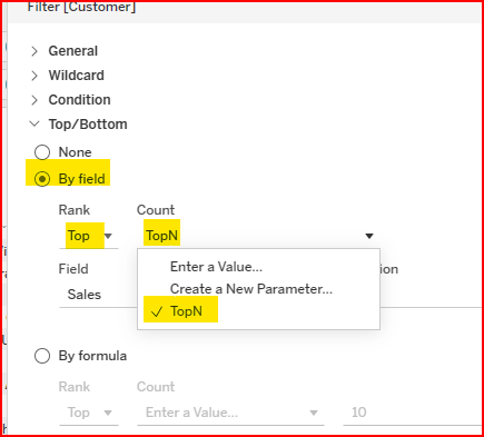
Filtering the Top N Members. Two methods:
-
Create a parameter named Top N, with Type = Integer.
-
Create a Sales by Customer view with the Rank Table Calculation and save the table calculation as a separate measure.
-
Method 1: Create a
-
Add the Customer Dimension to the Filters section. Select the Top/Bottom property and configure using the
TopNParameter to limit the number selection, based on the Sum of theSalesMeasure.
-
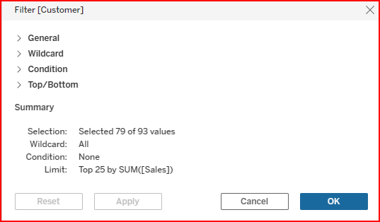
Tip: The difference between using the Top/Bottom Dimension Filter (above) and using the Rank(SUM(Sales)) Table Calculation Filter (below) is in how the Grand Totals display.
Grand Totals are calculated separately from the data section of the view. The Totals calculation looks at the Data filters, not Table Calculation filters. With the Table Calculation Filter, the Grand Total will be for all records selected by Dimension Filters and won’t match the sum of the rows displayed by the Table Calculation Filter.
Note: The Top/Bottom Dimension Filter might select different records than the Table Calculation Filter. I currently do not know why.
-
Create a calculated field: RANK(SUM([Sales]))<=[Top N]
-
Add the parameter to the report title (Insert → Parameter name).
-
Ex.: Top <Parameters.Top N> <Sheet Name> by Sales
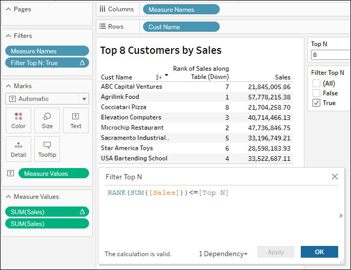
Note with Table Calc Filter, the Grand Totals don’t match the sum of the rows.
-
-
Parameter Controlling the Measure of a Report
-
Create a parameter named Select Measure, with Type = String, Allow values = List, create two values = Sales, GP. See below.
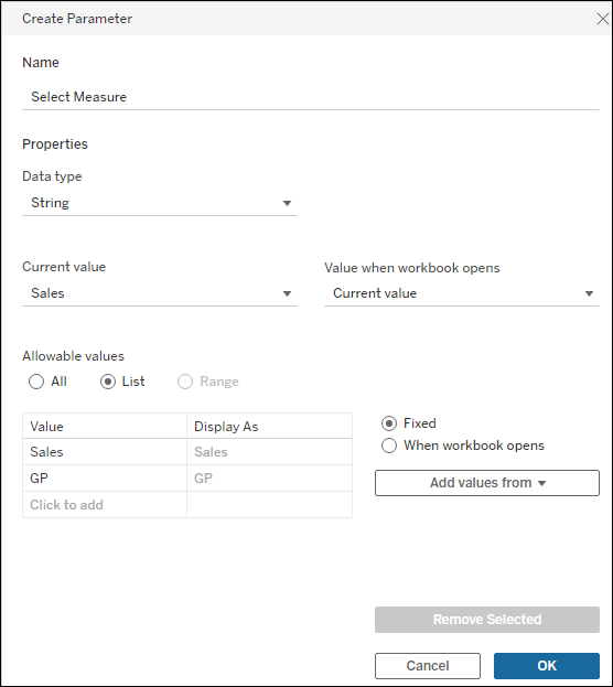
-
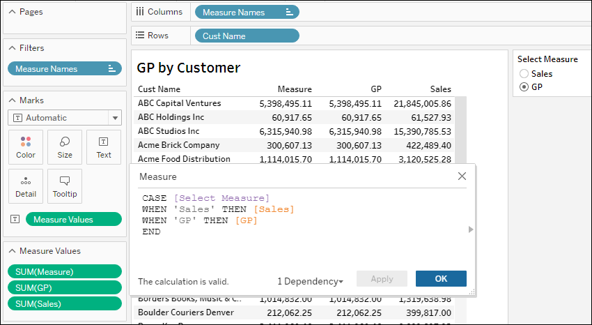
Create a calculated field and name it Measure:
-
CASE [Select Measure]
WHEN 'Sales' THEN [Sales]
WHEN 'GP' THEN [GP]
END
-
-
Create a report showing Measure, Sales and GP by Customer (see below).
-
Add the parameter to the report title (Insert → Parameter name).
-
Ex.: <Parameters.Select Measure> by <Sheet Name>
-
-
Change the parameter drop down to see that the new calculated field changes accordingly.
-
To change the Parameter to a radio button selector like below, go to the top right of the Parameter on the right panel, click the arrow down → Single Value (list).
-
-
4. Level of Detail (LOD)
One common use of LOD is the need to work with data that has been aggregated to different levels of detail.
LODs can be complex to understand and use, but they are powerful for many reporting needs. We’re going to cover one example here and provide documentation for further learning.
An Example of LOD
Build a report for Sales by Customer, % of total sales by Customer, and % of total sales by Cust Cat.
See the image below showing this report:
-
“% of Total Sales along Table (down)” = Quick Tableau Calculation (seen in the prior section).
-
Sales = regular Sales measure.
-
LOD expression = Cust Cat Total = {FIXED [Cust Cat]: SUM([Sales])}
-
Note that the sales aggregation is constant for each Cust Cat. This column is showing here to illustrate the concept.
-
Quick LOD:
-
Control-click the measure you want to aggregate and drag it to the dimension you want to aggregate on. A new field will appear with a new FIXED LOD calculation.
-
As a second option, select the measure you want to aggregate and then Control-click (or Command-click on a Mac) to select the dimension you want to aggregate on.
-
Right-click on the selected fields and select Create > LOD Calculation.
-
-
-
% Cust Cat Sales = SUM([Sales]) / MAX([Cust Cat Total])
-
In a real report, this calculated field can also incorporate the LOD expression and thus removing the need to show the Cust Cat Total column:
-
SUM([Sales]) / MAX({FIXED [Cust Cat]: SUM([Sales])})
-
-
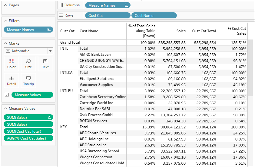
Tableau Help:
LODs and Filters:
FIXED LODs ignore report filters unless they are set to “Add to Context”
5. Dashboard Hands On Exercise
(self service only, not part of online training)
Using the techniques covered so far, let’s build a dashboard with the following specs:
-
Last 3 fiscal years
-
A user-entry parameter to set sales through a given fiscal month
-
A grid report showing Sales, YoY Monthly Var % and YTD
-
A chart for each of the measures
Click the following YouTube video to watch the dashboard creation: https://youtu.be/KRHYYX-MHh4
And here’s a screenshot of the desired dashboard:
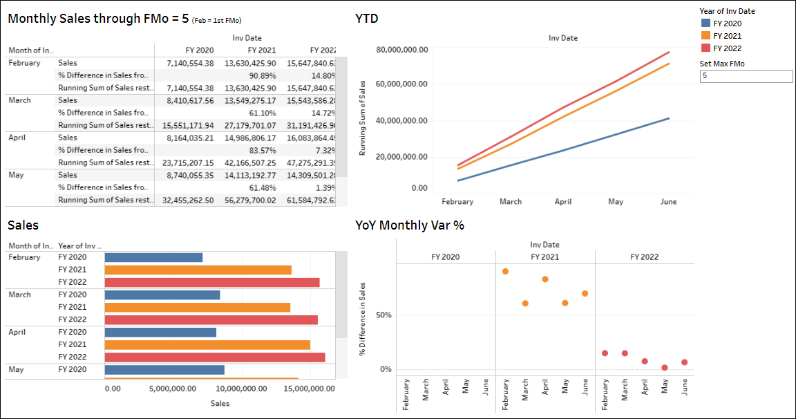
Grid Report
See text and video above for instructions:
-
Step 1: Sales by Year and Month.
-
Drag Inv Date to Columns.
-
Drag Inv Date to Rows → blue pill arrow down → Month May.
-
Drag Sales into report abc area.
-
-
Step 2: Set filter for the last 3 FYears
-
Drag Inv Date Options > FYr 0 = This Year into the Filters section. Select 0, -1 and -2 values.
-
Another way to do the same filter: drag Inv Date into the Filters section → click the arrow down on the top-right of the filter card on the right panel → Relative Date → click the filter Today value → Years → Last 3 years.
-
-
Step 3: Create parameter Set Max FMonth
-
Click arrow down by the Search box on the Data panel → Create Parameter.
-
Name it Set Max FMo → Integer type → Current value = 5 → Ok.
-
-
Step 4: Create calculated field for FMonth filtering.
-
Click arrow down by the Search box on the Data panel → Create Calculated Field.
-
Name it Filter FMo → enter expression [FMonth No]<=[Set Max FMo] → Ok.
-
-
Step 5: Create a filter with the new calculated field.
-
Drag Filter FMo to the Filters section → set it to True on the right panel.
-
-
Step 6: Quick Table Calculations for YTD and YoY Mo Var %.
-
Click arrow down on the Sales green pill → Quick Table Calculation → YTD.
-
Drag Sales onto the report numbers (this will add monthly Sales to YTD Sales report).
-
Turning the new monthly Sales into Percentage Difference: Click arrow down on the Sales green pill (the one without the triangle icon; triangle icon = table calculation) → Quick Table Calculation → Percent Difference.
-
Drag Sales onto the report numbers. This add monthly Sales onto the report.
-
On the green pills section, using drag-and-drop the green pills, order top to bottom: Sales, % Difference in Sales, Running Sum of Sales.
-
-
Step 7: More informative report title:
-
Right-click the tab on the bottom left → Rename to Monthly Sales.
-
Click the arrow down on the report title → Edit Title → enter the following:
-
<Sheet Name> through FMo = <Parameters.Set Max FMo> (1st FMo=Feb)
-
Ok.
-
-
Sales by Month with Bars
-
Drag Inv Date to Rows. Expand Year → Quarter → Month. Remove Quarter.
-
Drag Sales to Columns.
-
On the Marks section, change the dropdown from Automatic to Bars.
-
To apply the filters created in the prior report to this whole workbook, go back to the prior report tab, click the arrow down on each filter on the Filters section → Apply to Worksheets → All Using This Data Source. Go back to the tab where you’re building the cart report.
-
On Rows, drag Year to the right of Month.
-
Drag Inv Date onto the Color mark.
-
Rename the tab: right-click its tab → Rename = Monthly Sales Chart.
YTD Trend Lines
-
Drag Inv Date to Columns → click its blue pill’s arrow down → Month (May).
-
Drag Sales to Rows.
-
Drag Inv Date onto the Color mark.
-
Turning Sales into YTD: click the Sales green pill’s arrow down → Quick Table Calculation → YTD Total.
-
Rename the tab: right-click its tab → Rename = YTD.
YoY Monthly Variance %
-
Drag Inv Date to Columns → expand to Month, remove Quarter.
-
Drag Sales to Rows.
-
Drag Year to the right of Months in Columns.
-
Change Marks dropdown to Bars.
-
Turning Sales into YoY Monthly Var %:
-
Click the Sales green pill’s arrow down → Quick Table Calculation → Percent Difference. This calculation isn’t doing YoY Monthly Var % yet. Let’s edit it calculation.
-
Click the Sales green pill’s arrow down → Edit Table Calculation.
-
Set Percent Difference From → Specific Dimension → uncheck Month of the Inv Date.
-
Close the pop up.
-
-
Change Marks dropdown to Circles.
-
Drag Inv Date onto the Colors mark.
-
Rename the tab: right-click its tab → Rename = YoY Monthly Var %.
Dashboard Design
-
Click the Dashboard icon on the bottom row.
-
Click Size and change Fixed Size → Automatic.
-
Drag Monthly Sales sheet on the left panel onto the dashboard area.
-
Drag Monthly Sales Chart sheet at the bottom of the dashboard area.
-
Drag YTD sheet on the top right of the dashboard area.
-
Drag YoY Monthly Var % sheet on the bottom right of the dashboard area.
-
Click File → Save As to save your work.
Click the following YouTube video to watch the dashboard creation: https://youtu.be/KRHYYX-MHh4